Decoding 5-qubit perfect code#
In this experiment, we decode the 5-qubit code using mdopt. Here, we demonstrate direct-error input decoding, which means that the decoder takes a Pauli error as input and outputs the most likely logical operator. This pipeline is sufficient for threshold computation. After each run, the algorithm yields a probability distribution over the Pauli operators (I, X, Z, Y) to apply to the encoded logical qubit.
[1]:
import numpy as np
import qecsim.paulitools as pt
import matplotlib.pyplot as plt
from matplotlib import colormaps
from matplotlib.colors import LogNorm, Normalize
from matplotlib.ticker import FuncFormatter, FormatStrFormatter
from tqdm import tqdm
from scipy.stats import sem

from mdopt.mps.utils import create_custom_product_state
from mdopt.contractor.contractor import mps_mpo_contract
from mdopt.optimiser.utils import (
    apply_constraints,
    SWAP,
    COPY_LEFT,
    XOR_BULK,
    XOR_LEFT,
    XOR_RIGHT,
)

from examples.decoding.decoding import (
    custom_code_checks,
    custom_code_logicals,
    custom_code_logicals_sites,
    custom_code_constraint_sites,
    apply_bitflip_bias,
    apply_depolarising_bias,
    pauli_to_mps,
    decode_custom,
    css_code_stabilisers,
    multiply_pauli_strings,
    map_distribution_to_pauli,
    generate_pauli_error_string,
)
from examples.decoding.visualisation import plot_parity_check_mpo
Let us first define the code. Here, we won’t be using qecstruct as in the other examples because it lacks the machinery we need. Instead, we define the code as a list of stabilizers and logical operators.
[2]:
stabilizer_generators = [
    "XZZXI",
    "IXZZX",
    "XIXZZ",
    "ZXIXZ",
]
x_logical_operators = [
    "XXXXX",
]
z_logical_operators = [
    "ZZZZZ",
]
logical_operators = x_logical_operators + z_logical_operators
num_qubits = len(stabilizer_generators[0])
Let us first take a look at the code in terms of the MPS sites where the checks will be applied.
[3]:
checks = custom_code_checks(stabilizer_generators, logical_operators)

print("Stabilizer generators:")
for check in checks:
    print(check)
Stabilizer generators:
[2, 5, 7, 8]
[4, 7, 9, 10]
[2, 6, 9, 11]
[3, 4, 8, 11]
We now transform this into lists of sites where all the logical constraints are applied.
[4]:
constraint_sites = custom_code_constraint_sites(
    stabilizer_generators, logical_operators
)

print("MPS constraint sites:")
for string in constraint_sites:
    print(string)
MPS constraint sites:
[[2], [5, 7], [3, 4, 6], [8]]
[[4], [7, 9], [5, 6, 8], [10]]
[[2], [6, 9], [3, 4, 5, 7, 8, 10], [11]]
[[3], [4, 8], [5, 6, 7, 9, 10], [11]]
[5]:
logicals = custom_code_logicals(x_logical_operators, z_logical_operators)

print("Logical operators:")
print(logicals[0])
print(logicals[1])
Logical operators:
[[2, 4, 6, 8, 10]]
[[3, 5, 7, 9, 11]]
[6]:
logicals_sites = custom_code_logicals_sites(x_logical_operators, z_logical_operators)

print("MPS logical constraint sites:")
print(logicals_sites[0])
print(logicals_sites[1])
MPS logical constraint sites:
[[[0], [2, 4, 6, 8], [1, 3, 5, 7, 9], [10]]]
[[[1], [3, 5, 7, 9], [2, 4, 6, 8, 10], [11]]]
This quantum error correcting code is defined on \(5\) physical qubits and has \(2\) logical operators because it encodes \(1\) logical qubit. This means we will need \(5*2 + 2 = 12\) sites in our MPS.
[7]:
num_logicals = len(x_logical_operators) + len(z_logical_operators)
num_sites = 2 * len(stabilizer_generators[0]) + num_logicals

assert num_sites == 12
assert num_logicals == 2
Now, let us define the initial state. First of all we will check that no error implies no correction. This means starting from the all-zero state followed by decoding will return the all-zero state for the logical operators (the final logical operator will thus be identity operator). Thus, we start from the all-zero state for the error and the \(|+\rangle\) state for the logicals.
[8]:
error_state = "0" * (num_sites - num_logicals)
logicals_state = "+" * num_logicals
state_string = logicals_state + error_state
error_mps = create_custom_product_state(
    string=state_string, tolerance=1e-17, form="Right-canonical"
)
The lists of sites in the previous cells identify the sites where we will apply the XOR constraints. However, the MPOs will also consist of other tensors, such as SWAPs (a.k.a. the tensors’ legs crossings) and boundary XOR constraints. In what follows, we define the list of these auxiliary tensors.
[9]:
constraints_tensors = [XOR_LEFT, XOR_BULK, SWAP, XOR_RIGHT]
logicals_tensors = [COPY_LEFT, XOR_BULK, SWAP, XOR_RIGHT]
Now the fun part, MPS-MPO contraction. But first, we apply the bias channel to our error state. This is done to bias our output towards the received input. This is done by distributing the amplitude around the initial basis product state to other basis product states in the descending order by Hamming distance.
[10]:
renormalise = True
sites_to_bias = list(range(num_logicals, num_sites))
error_mps = apply_bitflip_bias(
    mps=error_mps,
    prob_bias_list=0.01,
    sites_to_bias=sites_to_bias,
)
[11]:
entropies, bond_dims = [], []

# for the X and the Z logicals
for i in [0, 1]:
    error_mps, entrps, bnd_dims = apply_constraints(
        error_mps,
        logicals_sites[i],
        logicals_tensors,
        cut=1e-17,
        chi_max=1e4,
        renormalise=renormalise,
        strategy="Optimised",
        return_entropies_and_bond_dims=True,
    )
    entropies += entrps
    bond_dims += bnd_dims

# for the stabilizer checks
error_mps, entrps, bnd_dims = apply_constraints(
    error_mps,
    constraint_sites,
    constraints_tensors,
    cut=1e-17,
    chi_max=1e4,
    renormalise=renormalise,
    strategy="Optimised",
    return_entropies_and_bond_dims=True,
)
entropies += entrps
bond_dims += bnd_dims
100%|██████████| 1/1 [00:00<00:00, 161.76it/s]
100%|██████████| 1/1 [00:00<00:00, 133.74it/s]
100%|██████████| 4/4 [00:00<00:00, 128.54it/s]
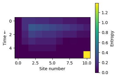
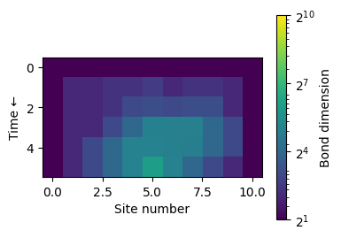
Let us now take a look at how the bond dimensions and entropies behave throughout the decoding process while applying the parity checks.
[12]:
plt.figure(figsize=(4, 3))
plt.imshow(entropies, cmap="viridis")
plt.colorbar(label="Entropy")
plt.xlabel("Site number")
plt.ylabel("Time ←")
plt.show()
[13]:
plt.figure(figsize=(4, 3))
plt.imshow(bond_dims, cmap="viridis", norm=LogNorm(vmin=2**1, vmax=2**10))
cbar = plt.colorbar(
    label="Bond dimension",
    format=FuncFormatter(lambda x, pos: f"$2^{{{int(np.log2(x))}}}$"),
    ticks=[2**i for i in range(1, 11, 3)],
)
plt.ylabel("Time ←")
plt.xlabel("Site number")
plt.show()
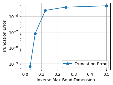
Let’s now take a look at how the truncation error behaves for different bond dimension cutoffs. First, let’s look at the bond dimensions appearing in the MPS if we do not impose any truncation.
[14]:
print(error_mps.bond_dimensions)
[2, 4, 8, 16, 32, 64, 32, 16, 8, 4, 2]
[15]:
bond_dims = [np.inf, 128, 64, 32, 16, 8, 4, 2]
inv_bond_dims = [1 / bd for bd in bond_dims]
errors = []
for chi in tqdm(bond_dims):
    errors.append(
        np.linalg.norm(
            error_mps.compress(
                chi_max=chi, renormalise=True, return_truncation_errors=True
            )[1]
        )
    )
100%|██████████| 8/8 [00:00<00:00, 24.25it/s]
[16]:
plt.figure(figsize=(4, 3))
plt.plot(inv_bond_dims, errors, marker="o", label="Truncation Error")
plt.xlabel("Inverse Max Bond Dimension")
plt.ylabel("Truncation Error")
plt.grid(True)
plt.yscale("log")
plt.legend()
plt.show()
Now, we marginalise over the message bits to get the probability distribution over the four possibilities of a logical operator: \(I\), \(X\), \(Z\), \(Y\).
[17]:
sites_to_marginalise = list(range(num_logicals, len(error_state) + num_logicals))
logical = error_mps.marginal(sites_to_marginalise=sites_to_marginalise)
logical = logical.dense(flatten=True, renormalise=True)
print(logical)
[0.9999731 0.00513518 0.00513518 0.0010249 ]
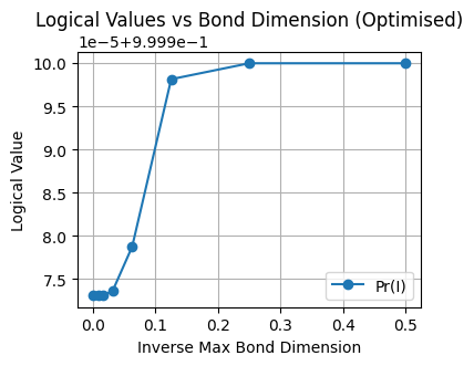
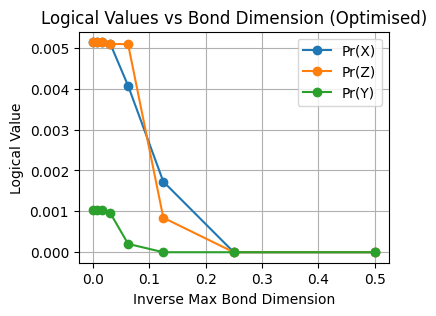
For the record, we’re hunting for the most likely logical operator to be the identity operator. So that’s it, we see the biggest probability assigned to the identity operator. Let’s see how the probabilities of the four operators change as we change the bond dimension cutoff.
[18]:
strategy = "Optimised"
logical_values = [[] for _ in range(4)]

for max_bond_dim in tqdm(bond_dims):
    error_state = "0" * (num_sites - num_logicals)
    logicals_state = "+" * num_logicals
    state_string = logicals_state + error_state
    error_mps = create_custom_product_state(string=state_string)

    error_mps = apply_bitflip_bias(
        mps=error_mps,
        prob_bias_list=0.01,
        sites_to_bias=sites_to_bias,
    )
    for i in [0, 1]:
        error_mps = apply_constraints(
            error_mps,
            logicals_sites[i],
            logicals_tensors,
            renormalise=renormalise,
            strategy=strategy,
            chi_max=max_bond_dim,
            silent=True,
            cut=1e-17,
        )
    error_mps = apply_constraints(
        error_mps,
        constraint_sites,
        constraints_tensors,
        renormalise=renormalise,
        strategy=strategy,
        chi_max=max_bond_dim,
        silent=True,
        cut=1e-17,
    )

    sites_to_marginalise = list(range(num_logicals, len(error_state) + num_logicals))
    logical = error_mps.marginal(sites_to_marginalise=sites_to_marginalise)
    logical = logical.dense(flatten=True, renormalise=True)

    for i in range(4):
        logical_values[i].append(logical[i])
100%|██████████| 8/8 [00:00<00:00, 44.33it/s]
[19]:
plt.figure(figsize=(4, 3))
plt.plot(inv_bond_dims, logical_values[0], marker="o", label=f"Pr(I)")
plt.xlabel("Inverse Max Bond Dimension")
plt.ylabel("Logical Value")
plt.title("Logical Values vs Bond Dimension (Optimised)")
plt.grid(True)
plt.legend()
plt.show()
[20]:
plt.figure(figsize=(4, 3))
plt.plot(inv_bond_dims, logical_values[1], marker="o", label=f"Pr(X)")
plt.plot(inv_bond_dims, logical_values[2], marker="o", label=f"Pr(Z)")
plt.plot(inv_bond_dims, logical_values[3], marker="o", label=f"Pr(Y)")
plt.xlabel("Inverse Max Bond Dimension")
plt.ylabel("Logical Value")
plt.title("Logical Values vs Bond Dimension (Optimised)")
plt.grid(True)
plt.legend()
plt.show()
Let’s now put all of this into a function. We’ll need this to run the decoder over a bunch of single- and multiqubit errors. For this, we first generate all possible one-, two- and three-qubit errors using qecsim.
[21]:
one_qubit_paulis = pt.ipauli(n_qubits=num_qubits, min_weight=1, max_weight=1)
two_qubit_paulis = pt.ipauli(n_qubits=num_qubits, min_weight=2, max_weight=2)
three_qubit_paulis = pt.ipauli(n_qubits=num_qubits, min_weight=3, max_weight=3)
[22]:
one_qubit_outputs = [
    decode_custom(
        stabilizers=stabilizer_generators,
        x_logicals=x_logical_operators,
        z_logicals=z_logical_operators,
        error=error,
        chi_max=1e4,
        cut=1e-10,
        tolerance=1e-10,
        bias_prob=0,
        silent=True,
    )
    for error in tqdm(one_qubit_paulis)
]
one_qubit_corrections_distribution = [output[0] for output in one_qubit_outputs]
15it [00:00, 84.47it/s]
[23]:
two_qubit_outputs = [
    decode_custom(
        stabilizers=stabilizer_generators,
        x_logicals=x_logical_operators,
        z_logicals=z_logical_operators,
        error=error,
        chi_max=1e4,
        cut=1e-10,
        tolerance=1e-10,
        bias_type="Depolarising",
        bias_prob=1e-2,
        silent=True,
    )
    for error in tqdm(two_qubit_paulis)
]
two_qubit_corrections_distribution = [output[0] for output in two_qubit_outputs]
90it [00:03, 26.20it/s]
[24]:
three_qubit_outputs = [
    decode_custom(
        stabilizers=stabilizer_generators,
        x_logicals=x_logical_operators,
        z_logicals=z_logical_operators,
        error=error,
        chi_max=1e4,
        cut=1e-10,
        tolerance=1e-10,
        bias_type="Depolarising",
        bias_prob=1e-2,
        silent=True,
    )
    for error in tqdm(three_qubit_paulis)
]
three_qubit_corrections_distribution = [output[0] for output in three_qubit_outputs]
270it [00:08, 33.25it/s]
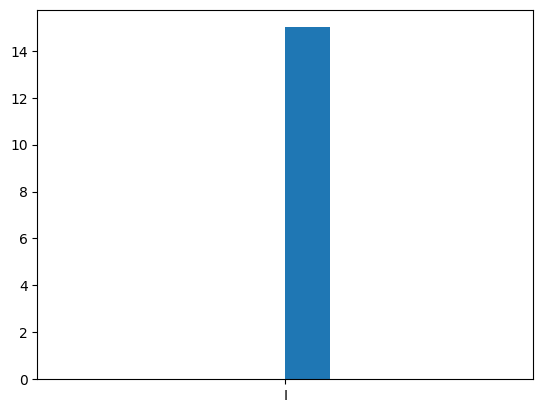
[25]:
plt.hist(map_distribution_to_pauli(one_qubit_corrections_distribution))
plt.show()
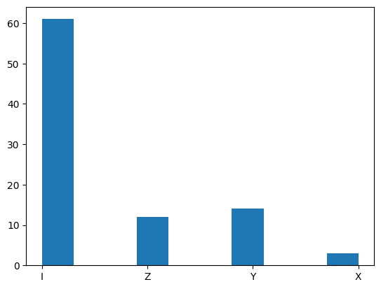
[26]:
plt.hist(map_distribution_to_pauli(two_qubit_corrections_distribution))
plt.show()
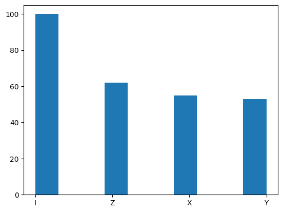
[27]:
plt.hist(map_distribution_to_pauli(three_qubit_corrections_distribution))
plt.show()
Let’s now check by hand that some of the decoder’s nontrivial outputs are indeed correct. First of all, from all one-qubit errors we get the Identity operator which corresponds to the fact that the 5-qubit code corrects all one-qubit errors. However, this code can also correct some two-qubit errors.
[28]:
one_qubit_paulis = list(pt.ipauli(n_qubits=num_qubits, min_weight=1, max_weight=1))
two_qubit_paulis = list(pt.ipauli(n_qubits=num_qubits, min_weight=2, max_weight=2))
three_qubit_paulis = list(pt.ipauli(n_qubits=num_qubits, min_weight=3, max_weight=3))
Let’s take a look at the errors which result in the Identity logical operator as the output.
[29]:
for i, correction in enumerate(
    map_distribution_to_pauli(two_qubit_corrections_distribution)
):
    if correction == "I":
        print(two_qubit_paulis[i])
XXIII
XZIII
XYIII
ZXIII
ZZIII
ZYIII
YXIII
YZIII
XIXII
XIZII
ZIXII
ZIZII
YIXII
YIZII
XIIXI
XIIZI
XIIYI
ZIIXI
ZIIZI
ZIIYI
YIIXI
YIIZI
YIIYI
XIIIX
XIIIZ
ZIIIX
ZIIIZ
YIIIX
YIIIZ
YIIIY
IXXII
IXZII
IXYII
IZXII
IZZII
IYZII
IXIXI
IXIZI
IXIYI
IZIXI
IZIZI
IYIZI
IXIIX
IZIIX
IZIIZ
IYIIX
IIXXI
IIXZI
IIXYI
IIZXI
IIZZI
IIYZI
IIXIX
IIXIZ
IIZIX
IIZIZ
IIYIZ
IIIXX
IIIXZ
IIIZX
IIIZZ
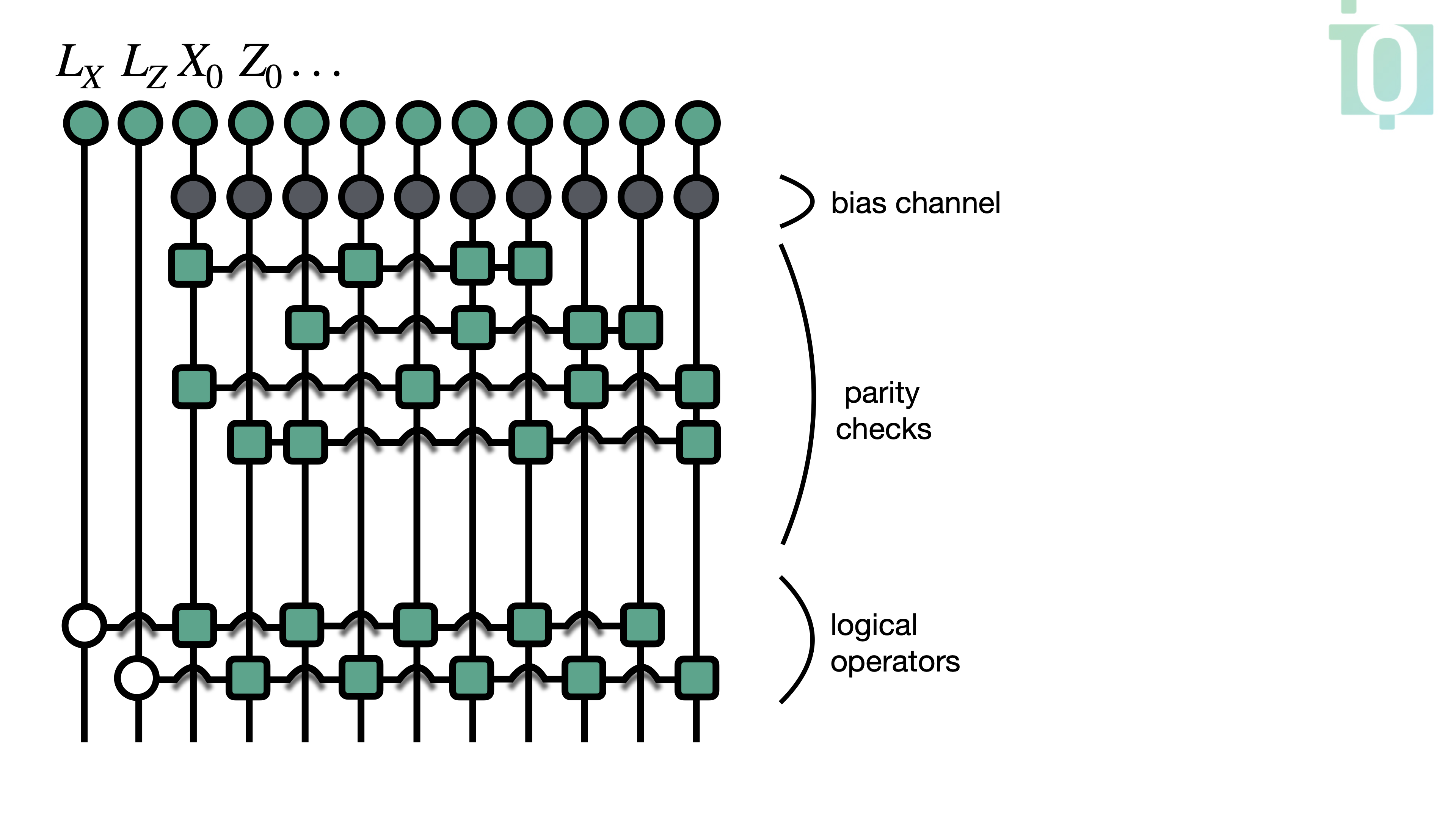
We now dive a bit more into what is happening inside the decoder to be able to better understand the results. For example, the first error \((X_0 X_1)\) from the list above would triggers all the parity checks. This can be seen from the actual tensor network we are building (see the image below). However, in the current setup the stabilisers are being set to \(0\), which is the result of the fact that the \(\text{XOR}\) tensors we use project out the inputs of odd (i.e., equal to \(1\)) parity. After applying the logical-operator MPOs and performing marginalization, the process yields a marginal distribution over codewords, each reflecting different parities of the logical operators.
Perfect, so we see how the failure rate goes down with the bond dimension.